Vector Random Variables
[!IMPORTANT]
A vector random variable is a vector whose components are random variables, often studied together to capture their joint statistical properties.
Let $\vec{X} = (X_1, X_2, ..., X_n)$, where each $X_i$ is a random variable defined on a common probability space. Such a collection is called a vector random variable or a random vector.
Example:
Consider the position of a moving particle in 2D space at time $t$, given by $\vec{X}(t) = (X_1(t), X_2(t))$, where $X_1$, $X_2$ are random variables denoting $x$ and $y$ coordinates.
[!NOTE]
In probability theory, most signal models, noise representations, and multichannel systems are naturally described using vector random variables.
Joint Distribution Function and its Properties
Definition of Joint CDF
[!IMPORTANT]
The joint cumulative distribution function (joint CDF) of two random variables $X$ and $Y$ is defined as $F_{XY}(x,y) = P(X \leq x, Y \leq y)$.
For $n$ random variables:
$$ F_{X_1,X_2,...,X_n}(x_1,x_2,...,x_n) = P(X_1 \leq x_1, X_2 \leq x_2, ..., X_n \leq x_n) $$
Properties of the Joint CDF (Derivation Included)
-
Non-decreasing:
$F_{XY}(x, y)$ is non-decreasing in both $x$ and $y$.
-
Limits:
-
$\lim_{x \to -\infty} F_{XY}(x, y) = 0$
-
$\lim_{y \to -\infty} F_{XY}(x, y) = 0$
-
$\lim_{x, y \to \infty} F_{XY}(x, y) = 1$
-
-
Right-Continuity:
$F_{XY}(x, y)$ is right-continuous in both variables.
-
Probability in Rectangular Region:
For $a < b$, $c < d$,
$$ P(a < X \leq b,\, c < Y \leq d) = F_{XY}(b,d) - F_{XY}(a,d) - F_{XY}(b,c) + F_{XY}(a,c) $$
Derivation for Probability in Rectangle:
Let $A = (X \leq b, Y \leq d)$, etc.
By the inclusion–exclusion principle:
\[ P(a < X \leq b, c < Y \leq d) = P(X \leq b, Y \leq d) - P(X \leq a, Y \leq d) - P(X \leq b, Y \leq c) + P(X \leq a, Y \leq c) \]
So,
$$ \boxed{ P(a < X \leq b, c < Y \leq d) = F_{XY}(b,d) - F_{XY}(a,d) - F_{XY}(b,c) + F_{XY}(a,c) } $$
[!TIP]
Always check the limits and monotonicity when asked properties of CDF.
[DIAGRAM: CANVAS: Surface plot showing $F_{XY}(x, y)$ as a smooth, non-decreasing surface in the $(x, y)$-plane, with contours indicating probability levels, and arrows marking the rectangle $(a, b) \times (c, d)$ illustrating how the joint CDF computes probability inside this box.]
The diagram above visually represents a typical joint CDF surface and how the probability of a rectangle can be calculated using the differences of CDF values at its corners.
Marginal Distribution Functions
Definition and Explanation
[!IMPORTANT]
The marginal distribution of $X$ (marginal CDF/PDF), given a joint distribution of $(X, Y)$, is the probability distribution of $X$ alone, obtained by integrating (continuous) or summing (discrete) out the other variable.
For joint PDF $f_{XY}(x, y)$:
- Marginal PDF of $X$:
$$ f_X(x) = \int_{-\infty}^{+\infty} f_{XY}(x, y) \, dy $$
- Marginal CDF of $X$:
$$ F_X(x) = \lim_{y \to \infty} F_{XY}(x, y) $$
Numerical Example
Given: $f_{XY}(x, y) = 6xy$, $0 < x < 1$, $0 < y < 1$
Find marginal PDF of $X$.
Step 1: Integrate $f_{XY}(x, y)$ over $y$:
\[ f_X(x) = \int_{0}^{1} 6xy\, dy = 6x \int_{0}^{1} y\, dy \]
\[ = 6x \left[ \frac{y^2}{2} \right]_0^1 = 6x \times \frac{1}{2} = 3x \]
So,
$$ \boxed{f_X(x) = 3x,\quad 0 < x < 1} $$
[!TIP]
Always ensure the marginal PDF integrates to 1 over its support. It's an easy way for partial credit!
Conditional Distribution and Density
Point Conditioning
[!IMPORTANT]
Conditional PDF of $X$ given $Y = y$ is $f_{X|Y}(x|y) = \dfrac{f_{XY}(x, y)}{f_Y(y)}$ if $f_Y(y) > 0$.
Conditional CDF: $F_{X|Y}(x|y) = P(X \leq x | Y = y)$
Numerical Example
Given $f_{XY}(x, y) = 2$, $0 < x < y < 1$
Find $f_{X|Y}(x|y)$ for $Y = 0.8$, $0 < x < 0.8$.
Step 1: Find $f_Y(y)$
\[ f_Y(y) = \int_{x=0}^{x=y} f_{XY}(x, y) dx = \int_{0}^{y} 2\, dx = 2y \]
Step 2: Use conditional formula
\[ f_{X|Y}(x|y) = \frac{f_{XY}(x, y)}{f_Y(y)} = \frac{2}{2y} = \frac{1}{y} \]
for $0 < x < y < 1$
Thus, for $Y=0.8$:
\[ f_{X|Y}(x|0.8) = \frac{1}{0.8} = 1.25\ \text{for } 0 < x < 0.8 \]
[!TIP]
For conditional density, always check the support (where the joint PDF is non-zero).
Interval Conditioning
[!IMPORTANT]
The conditional CDF/PDF of $X$ given $Y$ in an interval $[a, b]$ is obtained by restricting $Y$ and normalizing.
Conditional PDF:
\[ f_{X\,|\,a<Y<b}(x) = \frac{\displaystyle \int_a^b f_{XY}(x, y)\, dy}{P(a < Y < b)} \]
where $P(a < Y < b) = \displaystyle \int_a^b f_Y(y) dy$
Applications:
-
Filtering signal/noise that matches some interval
-
Bayesian inference, etc.
Statistical Independence
Definition
[!IMPORTANT]
Two random variables $X$ and $Y$ are statistically independent if:
$$ > F_{XY}(x, y) = F_X(x) F_Y(y) \quad \text{and} \quad f_{XY}(x, y) = f_X(x) f_Y(y) > $$
Methods to Test Independence
-
Check if $f_{XY}(x, y)$ factorizes as $f_X(x) f_Y(y)$ for all $(x, y)$.
-
Compare joint and product of marginals for at least two $(x, y)$ pairs.
Numerical Example
Given: $f_{XY}(x,y) = 6xy$ for $0 < x < 1,\ 0 < y < 1$
From earlier, $f_X(x) = 3x$, $f_Y(y) = 3y$.
Do $f_{XY}(x, y) = f_X(x) f_Y(y)$?
\[ f_X(x) f_Y(y) = 3x \cdot 3y = 9xy \neq 6xy = f_{XY}(x, y) \]
So, $X$ and $Y$ are dependent.
[!TIP]
If the support is a rectangle and $f_{XY}(x, y)$ is a product, likely independent; otherwise not.
Sum of Two Random Variables
Distribution Definition
Given $Z = X + Y$, the distribution of $Z$ is derived from those of $X$ and $Y$.
Derivation: Density and Convolution Formula (Independent)
[!IMPORTANT]
For independent continuous $X$, $Y$, the PDF of $Z=X+Y$ is the convolution:
\[ f_Z(z) = \int_{-\infty}^{+\infty} f_X(x) f_Y(z - x) dx \]
Step-by-step Derivation:
-
PDF of $Z$:
\[ f_Z(z) = \frac{d}{dz} P(Z \leq z) = \frac{d}{dz}P(X + Y \leq z) \]
-
$P(X + Y \leq z) = \displaystyle\iint_{x+y \leq z} f_X(x) f_Y(y) dx\, dy$
-
Let $y = z-x$; express all in $x$:
\[ f_Z(z) = \int_{-\infty}^{+\infty} f_X(x) f_Y(z-x) dx \]
$
\boxed{f_Z(z) = \int_{-\infty}^{+\infty} f_X(x), f_Y(z-x), dx} $
Convolution Diagram
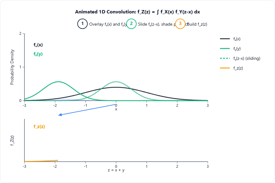
This diagram depicts how convolution merges two random variable PDFs to build the PDF of their sum.
Numerical Example
If $X$ and $Y$ are uniform on $(-1, 1)$, find the PDF of $Z = X+Y$.
Given: $f_X(x) = f_Y(y) = \frac{1}{2}$ for $-1 < x, y < 1$.
The range of $Z$ is $-2 < z < 2$.
\[ f_Z(z) = \int_{-\infty}^{+\infty} f_X(x) f_Y(z - x) dx \]
But $f_X(x)$ and $f_Y(z - x)$ are nonzero only when $-1 < x < 1$ and $-1 < z - x < 1$.
So, $x \in [\max(-1, z-1), \min(1, z+1)]$
Work out cases:
-
For $-2 < z < 0$, the limits are $x \in [-1, z+1]$
-
For $0 \leq z < 2$, $x \in [z-1, 1]$
Thus,
\[ f_Z(z) = \int_{\text{limits}} \frac{1}{2} \cdot \frac{1}{2} dx = \frac{1}{4} (\text{upper limit} - \text{lower limit}) \]
So
\[ f_Z(z) = \begin{cases} \frac{1}{4}(z+2), & -2 < z < 0\\ \frac{1}{4}(2-z), & 0 \leq z < 2 \end{cases} \]
Graph is triangular with peak at $z=0$.
[!TIP]
When asked for the distribution of $Z = X + Y$, always check and indicate the bounds for $z$.
Sum of Several Random Variables
Extension and Notation
Let $Z = X_1 + X_2 + ... + X_n$, where $X_i$ are independent.
\[ f_Z(z) = f_{X_1} * f_{X_2} * ... * f_{X_n}(z) \]
where $*$ is the convolution operator.
Practical Example (Numerical)
If $X_1, X_2, X_3$ are independent and uniform on $(0,1)$, what is $E[Z]$ and $Var(Z)$?
$
E[X_i] = \frac{1}{2},, Var(X_i) = \frac{1}{12} $
So,
\[ E[Z] = E[X_1] + E[X_2] + E[X_3] = \frac{3}{2} \]
\[ Var(Z) = Var(X_1) + Var(X_2) + Var(X_3) = \frac{3}{12} = \frac{1}{4} \]
Central Limit Theorem (CLT)
[!IMPORTANT]
The Central Limit Theorem states that the sum (or average) of a large number of independent, identically distributed random variables with finite mean $\mu$ and variance $\sigma^2$ approaches a normal (Gaussian) distribution, regardless of the original variable's distribution.
Mathematically, if $Z_n = \frac{\sum_{i=1}^n X_i - n\mu}{\sigma \sqrt{n}}$, then as $n \to \infty$
\[ Z_n \Longrightarrow \mathcal{N}(0, 1) \]
Applications:
-
Noise aggregation in communication systems
-
Sampling and measurement error analysis
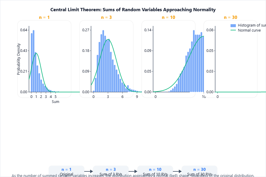
The figure shows the emergence of the normal curve as more independent variables are summed.
[!TIP]
For engineering exams, always mention that the CLT justifies the use of Gaussian models for noise!
Unequal Distribution, Equal Distributions
| Property | Equal/Identical Distributions | Unequal/Non-identical Distributions |
|---|---|---|
| Means / Variance | All $E[X_i]=\mu$ / $Var(X_i)=\sigma^2$ | Means/vars differ per variable |
| CLT applies? | Yes | Yes, if variances are all finite |
| Summation approach | Simple, repeat for all variables | Must track each $f_{X_i}$ separately |
| Expression for $E[Z]$ | $n\mu$ | $\sum_i E[X_i]$ |
| Expression for $Var(Z)$ | $n\sigma^2$ | $\sum_i Var(X_i)$ |
[!NOTE]
The sum of means/variances is always additive if variables are independent, regardless of identical distribution.
Expected Value of a Function of Random Variables
[!IMPORTANT]
The expected value of $g(X, Y)$ is:
\[ E[g(X, Y)] = \iint g(x, y) f_{XY}(x, y)\, dx\, dy \]
For discrete: $E[g(X, Y)] = \sum_x \sum_y g(x, y) P_{XY}(x, y)$
Numerical Example
Given $f_{XY}(x, y) = 6xy$, $0 < x < 1, 0 < y < 1$, find $E[XY]$.
\[ E[XY] = \int_0^1 \int_0^1 x y \cdot 6 x y\, dy\, dx = 6 \int_0^1 \int_0^1 x^2 y^2\, dy\, dx \]
\[ = 6 \int_0^1 x^2 dx \int_0^1 y^2 dy = 6 \left[ \frac{x^3}{3} \right]_0^1 \left[ \frac{y^3}{3} \right]_0^1 = 6 \times \frac{1}{3} \times \frac{1}{3} = \frac{2}{3} \]
Joint Moments about the Origin
[!IMPORTANT]
The joint moment of order $(r, s)$ about the origin is $E[X^r Y^s] = \iint x^r y^s f_{XY}(x, y)\, dx\, dy$ (or sum for discrete).
-
Zero order: $E[1] = 1$
-
First order: $E[X],\, E[Y]$
-
Second order: $E[X^2],\, E[Y^2],\,E[XY]$
Joint Central Moments
[!IMPORTANT]
The joint central moment of order $(r, s)$ is $E[(X - E[X])^r (Y - E[Y])^s]$.
- Covariance: $Cov(X, Y) = E[(X - E[X])(Y - E[Y])] = E[XY] - E[X]E[Y]$
Joint Characteristic Functions
[!IMPORTANT]
The joint characteristic function for $(X, Y)$ is $\phi_{XY}(w_1, w_2) = E[e^{j(w_1 X + w_2 Y)}]$
- Property: The joint characteristic function uniquely determines the joint distribution.
Jointly Gaussian Random Variables
Two Random Variables Case
[!IMPORTANT]
Two random variables $(X, Y)$ are jointly Gaussian if every linear combination $aX + bY$ is Gaussian.
The joint PDF:
\[ f_{XY}(x, y) = \frac{1}{2\pi \sigma_X \sigma_Y \sqrt{1 - \rho^2}} \exp\left( - \frac{1}{2(1 - \rho^2)} \left( \frac{(x - \mu_X)^2}{\sigma_X^2} - 2\rho \frac{(x - \mu_X)(y - \mu_Y)}{\sigma_X \sigma_Y} + \frac{(y - \mu_Y)^2}{\sigma_Y^2} \right) \right) \]
where $\rho$ is the correlation coefficient.
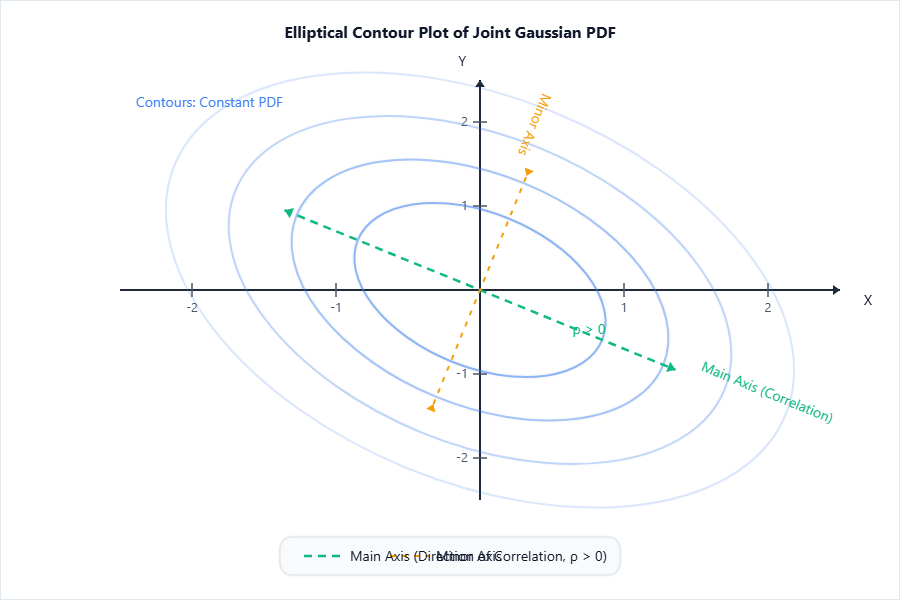
This diagram shows the typical "ridge" shape of correlated Gaussian distributions.
$n$ Random Variables Case and Properties
If $\vec{X}$ is $n$-dimensional, joint PDF is characterized by mean vector $\vec{\mu}$, covariance matrix $\Sigma$.
Main properties:
-
Any marginal of a jointly Gaussian vector is Gaussian.
-
Linear combinations are Gaussian.
-
Uncorrelated Gaussian variables are independent.
Transformations of Multiple Random Variables
General Method
[!IMPORTANT]
For transformation $(X, Y) \to (U, V)$, the joint PDF $f_{UV}(u, v)$ is given by:
\[ f_{UV}(u, v) = f_{XY}(x(u, v), y(u, v)) \cdot \left|J\right| \]
where $J$ is the Jacobian determinant of the transformation.
Jacobian Derivation (2D)
Let $u = g_1(x, y)$, $v = g_2(x, y)$. Inverse: $x = h_1(u, v), y = h_2(u, v)$.
Jacobian:
\[ J = \left| \begin{array}{cc} \frac{\partial x}{\partial u} & \frac{\partial x}{\partial v} \\ \frac{\partial y}{\partial u} & \frac{\partial y}{\partial v} \end{array} \right| \]
So,
\[ \boxed{ f_{UV}(u, v) = f_{XY}(x(u, v), y(u, v)) \times \left|J\right| } \]
Worked Example
Let $X$ and $Y$ be independent, uniform on $(0, 1)$. Let $U = X + Y$, $V = X - Y$.
We want $f_{UV}(u, v)$.
-
Invert:
\[ X = \frac{U + V}{2},\ \ Y = \frac{U - V}{2} \]
-
Jacobian:
\[ J = \left| \begin{array}{cc} \frac{\partial x}{\partial u} & \frac{\partial x}{\partial v} \\ \frac{\partial y}{\partial u} & \frac{\partial y}{\partial v} \end{array} \right| = \left| \begin{array}{cc} \frac{1}{2} & \frac{1}{2}\\ \frac{1}{2} & -\frac{1}{2} \end{array} \right| = \frac{1}{2} \times (-\frac{1}{2}) - \frac{1}{2} \times \frac{1}{2} = -\frac{1}{4} - \frac{1}{4} = -\frac{1}{2} \]
$|J| = \frac{1}{2}$
-
$f_{XY}(x, y) = 1$ for $0 < x < 1,\, 0 < y < 1$
So
\[ f_{UV}(u, v) = 1 \times \frac{1}{2} = \frac{1}{2} \]
with the correct region for $(u, v)$ given by inverse mapping of the rectangle $0 < X < 1,\ 0 < Y < 1$.
Linear Transformations of Gaussian Random Variables
[!IMPORTANT]
Any linear transformation of jointly Gaussian random variables yields another set of Gaussian random variables.
That is, if $\vec{Y} = A \vec{X} + \vec{b}$ for matrix $A$, vector $\vec{b}$, and $\vec{X}$ jointly Gaussian, then $\vec{Y}$ is jointly Gaussian.
Main properties
-
$E[\vec{Y}] = A E[\vec{X}] + \vec{b}$
-
$Cov(\vec{Y}) = A \, Cov(\vec{X}) \, A^T$
Numerical Example
Let $X, Y$ be independent $N(0, 1)$. Let $Z = 2X + 3Y$.
-
$E[Z] = 2E[X] + 3E[Y] = 0$
-
$Var(Z) = 2^2 Var(X) + 3^2 Var(Y) = 4 + 9 = 13$
-
Distribution: $Z \sim N(0, 13)$
END OF UNIT 3 EXAM-WINNING SHORT NOTES