Analysis Design of Algorithm (CS-402) Unit 6 Notes

Introduction

1. Binary Search Trees (BST)

Definition and Properties

[!IMPORTANT]

A Binary Search Tree (BST) is a binary tree in which for every node:

All nodes in the left subtree have keys less than the node’s key.

All nodes in the right subtree have keys greater than the node’s key.

Basic BST Terminology

Root: The topmost node.
Leaf: A node with no children.
Subtree: A tree consisting of a node and its descendants.

[!TIP]

In BSTs, keys are unique and allow efficient searching, insertion, and deletion.

BST Operations

Insertion Algorithm

To insert a value into a BST:

Start at the root.
If the tree is empty, create a new node and make it the root.
Otherwise, compare the value to insert ($x$) to the current node’s key ($K$):
- If $x < K$, go left.
- If $x > K$, go right.
- Repeat until a null position is found, then insert.

Pseudocode:


BST-Insert(T, x):

  if T is empty:

      create new node with key x, return as root

  else if x < T.key:

      T.left = BST-Insert(T.left, x)

  else if x > T.key:

      T.right = BST-Insert(T.right, x)

  return T

Time Complexity: $O(h)$, where $h$ is the height of the tree ($O(\log n)$ for balanced, $O(n)$ for skewed).

Numerical Example:

Insert 15, 10, 20, 8 into BST:

Insert 15 → root
Insert 10 ($10 < 15$) → left child of 15
Insert 20 ($20 > 15$) → right child of 15
Insert 8 ($8 < 15$, $8 < 10$) → left child of 10

BST Looks like:

Deletion Algorithm ⭐

There are three cases for deletion in a BST:

Node is a leaf: Remove the node.
Node has one child: Replace node with its child.
Node has two children:
- Find the inorder successor (minimum in right subtree) or predecessor (maximum in left subtree).
- Replace node’s value with successor’s (or predecessor's).
- Delete the successor (which will now be either a leaf or one child).

Detailed Algorithm:


BST-Delete(T, x):

  if T is null: return T

  if x < T.key:

      T.left = BST-Delete(T.left, x)

  else if x > T.key:

      T.right = BST-Delete(T.right, x)

  else:

      // Node found

      if T.left == null:

          return T.right

      else if T.right == null:

          return T.left

      else:

          // Two children - find inorder successor

          succ = Min(T.right)

          T.key = succ.key

          T.right = BST-Delete(T.right, succ.key)

  return T

Time Complexity: $O(h)$

Numerical Example:

Delete 10 from the BST:

10 has one child (8).
Replace 10 with 8.

Final tree:

[!TIP]

Always check all three cases and remember to update parent pointers in actual implementation.

Search Algorithm


BST-Search(T, x):

  if T is null or T.key == x: return T

  if x < T.key: return BST-Search(T.left, x)

  else: return BST-Search(T.right, x)

Time Complexity: $O(h)$

Time Complexities of BST Operations

Operation	Best Case	Average Case	Worst Case
Search	$O(\log n)$	$O(\log n)$	$O(n)$
Insert	$O(\log n)$	$O(\log n)$	$O(n)$
Delete	$O(\log n)$	$O(\log n)$	$O(n)$

Balanced BST: $h=\log n$
Unbalanced (Skewed) BST: $h = n$

2. Height-Balanced Trees (AVL Trees)

Definition and Properties

[!IMPORTANT]

An AVL tree is a self-balancing binary search tree where for any node, the heights of the left and right subtrees differ by at most 1.

AVL Tree Properties:

BST property holds.
Trees stay balanced after each insertion/deletion.

Balance Factor Concept ⭐

[!IMPORTANT]

Balance Factor (BF) of a node = Height(left subtree) − Height(right subtree)

For AVL: BF ∈ {$-1$, $0$, $1$} at every node.

Numerical Example:

Node $P$ with left subtree of height 2, right subtree of height 1:

$$ \text{BF}(P) = 2 - 1 = 1 $$

So the node is balanced.

AVL Condition

After every modify operation, all nodes must have BF $\in \{-1, 0, 1\}$.

Rotations in AVL Trees ⭐

Balancing is restored with rotations:

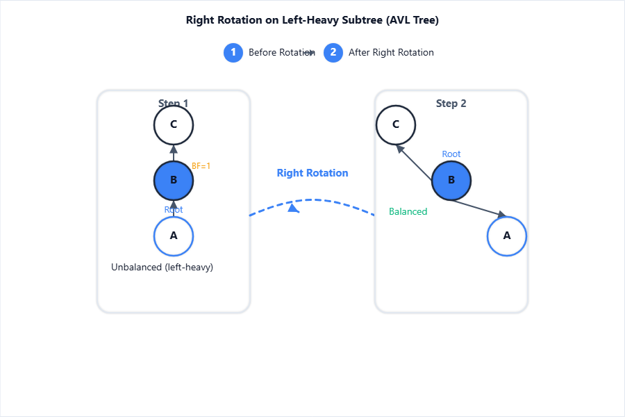
Single Right Rotation (LL Rotation)

Draw a subtree with node A (unbalanced, left-heavy) as root;

Before: Unbalanced at A due to insert in left subtree of left child.
After: B becomes new root; original root A becomes right child.

Description: Single right rotation restores AVL condition for a "left-left" case.

Single Left Rotation (RR Rotation)

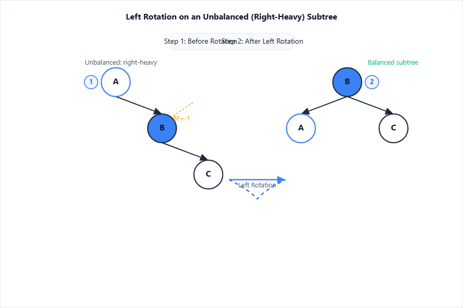
Draw a subtree with node A (unbalanced, right-heavy) as root

"Right-Right" case (insert in right subtree of right child).

Description: Single left rotation fixes "right-right" imbalance.

Double Rotations (LR & RL Rotations)

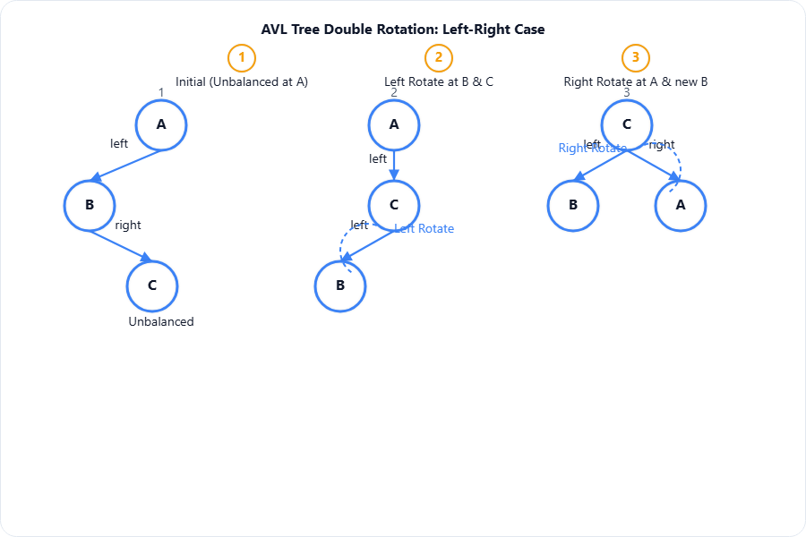
Left-Right (LR):

Node A (unbalanced to left child), left child B, B's right c

Right-Left (RL):

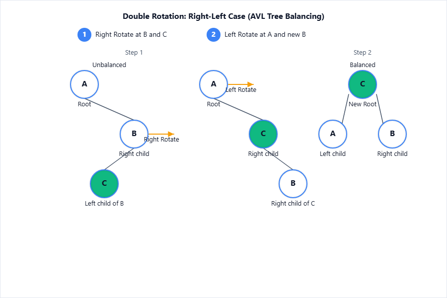
Node A (unbalanced to right child), right child B, B's left

Description: Double rotations are used if insertion/deletion causes imbalance in the “outer” grandchild.

[!TIP]

LL and RR — single rotation (when inserted in "outside" grandchild<br>

LR and RL — double rotation (when inserted in "inside" grandchild)

Example: Rotations

Insert $30$, $20$, $40$, $10$ into AVL.

$30$ → root
$20$ ($< 30$) → left of 30
$40$ ($> 30$) → right of 30
$10$ ($< 30$, $< 20$) → left of 20. Node 30’s BF = 2 (imbalance).

Apply single right rotation at 30.


   30                20

  /  \     =>       /  \
20   40           10   30

/
10                   \

                     40

AVL Operations

Insertion (with balancing)

Insert using BST logic.
Update balance factors on path up.
If any BF is not in $[-1, 0, 1]$, apply appropriate rotation(s).

Numerical Example:

Insert 50, 40, 30:

After 50:

After 40:

After 30: (Need LL rotation)

After right rotation at 50:

Deletion

After node removal, may need rotations if balance factors are disturbed.

Applications/Advantages

Search, insert, delete in $O(\log n)$ time.
Ideal for in-memory search (DBMS indices, file systems).
Trees remain always balanced.

3. 2–3 Trees and B-Trees

A. 2–3 Trees

Definition and Properties

[!IMPORTANT]

A 2–3 tree is a balanced search tree where each internal node has 2 or 3 children, and each node contains 1 or 2 keys.

Node Types:

2-Node: 1 key, 2 children
3-Node: 2 keys, 3 children

Properties:

All leaves are at the same depth (balanced).
Supports fast search (paths of similar length).

Insertion and Deletion

Steps for Insertion:

Insert at leaf node in key order.
If node overflows (3 keys), split into two nodes and move middle key to parent.
May recursively split up to root.

Numerical Example with Diagram:

Insert keys 10, 20, 30 into empty 2–3 tree:

10: [10]
20: [10, 20]
30: Node full, split: [20] becomes new root, [10] and [30] are children.

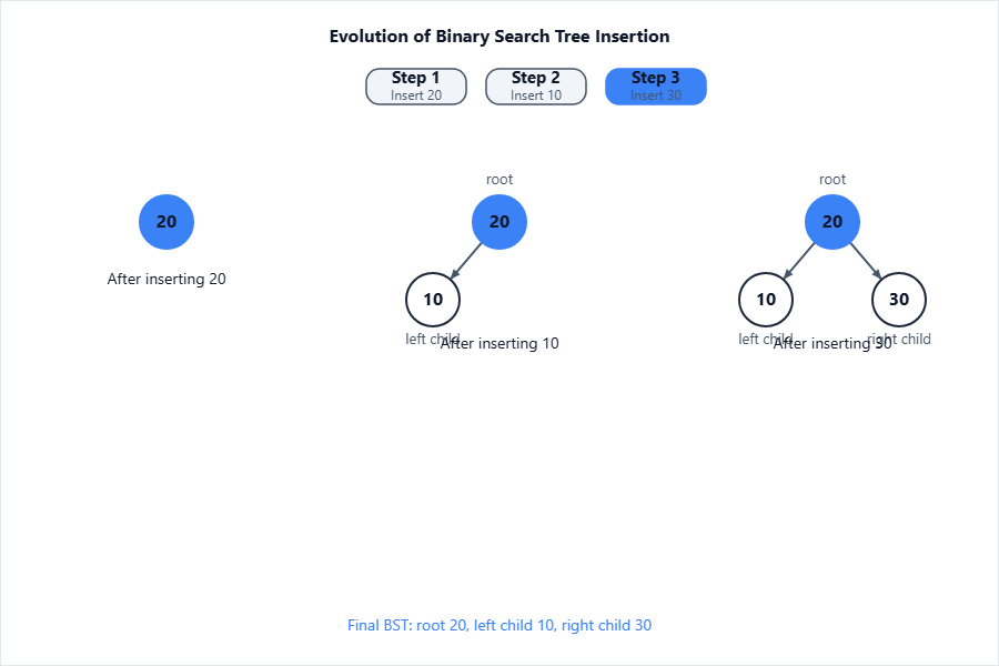
Show evolution of tree as each key is inserted, ending with

Description: After insertions, tree is perfectly balanced.

Use Cases / Applications

Used to implement associative arrays, database indices in memory.
Good for workloads with frequent insert/delete.

2–3 Trees vs BSTs

Feature	2–3 Tree	BST
Balanced	Always (height-balanced)	Not guaranteed
Search Time	$O(\log n)$	Average $O(\log n)$, Worst $O(n)$
Max node degree	3	2
Practical Usage	Used in DBMS, Storage	Used for fast lookup in RAM

[!TIP]

Limitation: 2–3 trees can be complex to implement due to node splitting and merging.

B. B-Trees

Definition and Properties

[!IMPORTANT]

A B-Tree of order $m$ (minimum degree $t$):

Each node may have at most $m$ children.

Each node (except root) has at least $\lceil m/2 \rceil$ children.

All leaves at the same depth.

Node contains $k$ keys ($\lceil m/2 \rceil-1 \leq k \leq m-1$).

Rules:

Internal nodes function like "blocks" with sorted keys—suitable for disk arrays.
Insertions and deletions keep the tree balanced by splitting/merging nodes.

Insertion Process

Start at root, find leaf for new key.
Insert key in order.
If node overflows, split into two and push middle key to parent.
If root overflows, create new root.

Numerical Example & Diagram:

Insert 5, 10, 15, 20 into B-tree of order 3 (max 2 keys per node):

Insert [5]
Insert [5, 10]
Insert [5, 10, 15]: node full, split to [10], left child [5], right child [15]
Insert 20: Insert into right child [15], result [15, 20] (no split needed)

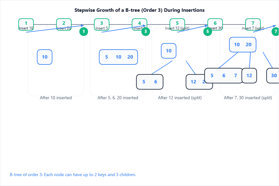
Stepwise growth of B-tree as each number is inserted.

Description: Each split causes tree to grow wider or taller, but always balanced.

B-Tree Construction (Order n)

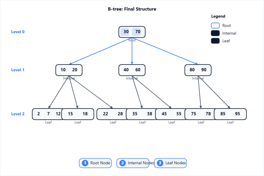
Given keys [2, 4, 6, 8, 10], order $n=3$:

Insert 2: [2]
4: [2, 4]
6: Node full, split [4] up, children [2], [6]
Insert 8: right child → [6, 8]
Insert 10: right child full, split up [8]. Tree becomes:

Root: [4, 8], children: [2], [6], [10]

B-tree in the above final structure.

Applications

File systems (NTFS, BtrFS, ext4 directories)
Database indexing (MySQL, PostgreSQL)
Efficient for large data blocks on disk

4. Tree Traversal Techniques (In‑order, Pre‑order, Post‑order)

Definitions and Use ⭐

[!IMPORTANT]

In-order: Visit left subtree, node, right subtree.

Pre-order: Visit node, left subtree, right subtree.

Post-order: Visit left subtree, right subtree, node.

Uses:

In-order: Sort BST values, reconstruct binary tree from traversals.
Pre-order: Copy tree, prefix expression evaluation.
Post-order: Delete/free tree, postfix expression evaluation.

Pseudocode / Stepwise Traversal

In-order:


Inorder(node):

  if node != null:

    Inorder(node.left)

    Visit(node)

    Inorder(node.right)

Pre-order:


Preorder(node):

  if node != null:

    Visit(node)

    Preorder(node.left)

    Preorder(node.right)

Post-order:


Postorder(node):

  if node != null:

    Postorder(node.left)

    Postorder(node.right)

    Visit(node)

Worked Example with Diagram

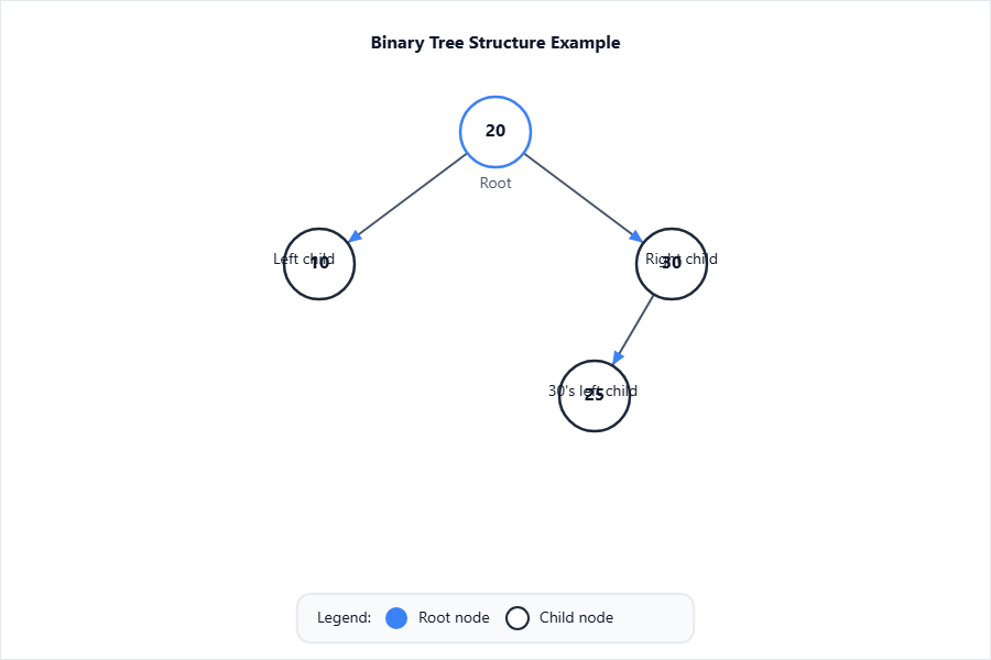
Consider tree:

Binary tree with root 20, left 10, right 30; 30's left child

In-order Traversal: Left, Root, Right
- 10, 20, 25, 30
Pre-order Traversal: Root, Left, Right
- 20, 10, 30, 25
Post-order Traversal: Left, Right, Root
- 10, 25, 30, 20

[!TIP]

Draw small trees and trace step by step in the exam for partial marks.

5. Graph Traversal Algorithms (DFS, BFS)

Definitions (DFS and BFS) ⭐

[!IMPORTANT]

Graph traversal means visiting all the vertices in a graph in a systematic order.

DFS: Follows one branch as deep as possible before backtracking.

BFS: Explores all neighbors at current depth before moving to next level.

Use cases:

DFS: Topological sort, connected components, maze solving.
BFS: Shortest paths in unweighted graph (e.g., AI/game moves).

DFS (Depth First Search) ⭐

Algorithm (Pseudocode):


DFS(v):

  Mark v as visited

  For each neighbor u of v:

    if u is not visited:

      DFS(u)

Can be implemented recursively or with explicit stack.

Recursion Depth:

Equals to max path length from start vertex to furthest node.

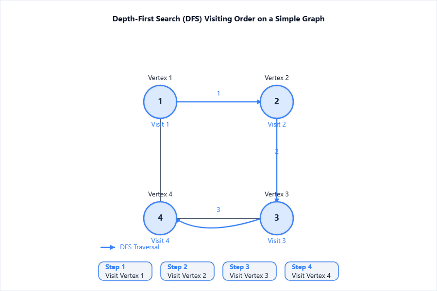
Simple graph with 4 vertices. Start DFS at vertex 1, show vi

DFS Example:

Given graph: 0—1, 0—2, 1—3

Start at 0:

Visit 0, 1, 3, 2 (One possible DFS order)

[!TIP]

DFS always finds all vertices reachable from the start vertex.

BFS (Breadth First Search) ⭐

Algorithm (Pseudocode):


BFS(s):

  Initialize queue Q

  Mark s as visited

  Enqueue s into Q

  while Q not empty:

    v = Dequeue Q

    for each neighbor u of v:

      if u not visited:

        Mark u as visited

        Enqueue u into Q

Uses a queue to explore vertices level by level.

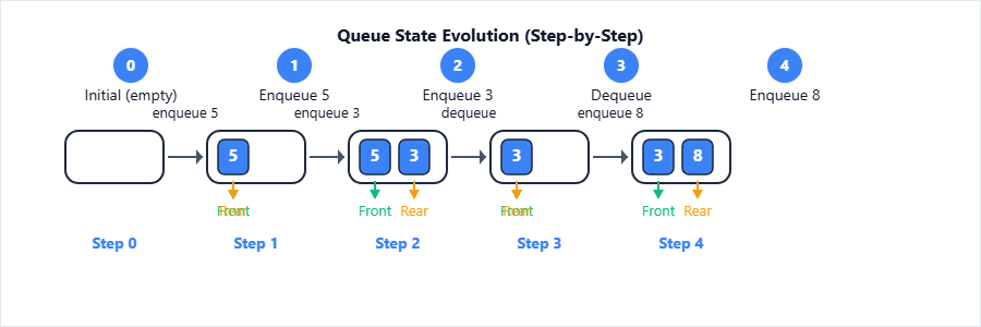
Small graph (like above). Show queue states at each step.

BFS Example:

Graph as above. Start at 0:

Order: 0, 1, 2, 3

BFS vs DFS (Comparison)

Feature	DFS	BFS
Data Structure	Stack (recursion/explicit)	Queue
Order	Deep before wide	Level by level
Space (sparse graph)	$O(h)$ (h=height/depth)	$O(w)$ (w=max width)
Finds Shortest Path	No	Yes (unweighted)
Applications	Topological, Comp. components	Shortest path, layer order

Applications/Properties

Both visit all reachable vertices ($O(V+E)$ time, $V$=vertices, $E$=edges).
Used in AI, compilers, operating systems, and social network analysis.

6. Fundamentals of NP‑Completeness

P (Polynomial Time) & NP (Nondeterministic Polynomial Time)

[!IMPORTANT]

P: Class of decision problems solvable by a deterministic Turing machine in polynomial time.

NP: Problems for which a solution can be verified in polynomial time by a deterministic Turing machine.

NP-Complete Problem Concept ⭐

[!IMPORTANT]

NP-Complete problems are problems in NP to which every other NP problem is polynomial-time reducible. If any NP-complete problem can be solved in polynomial time, all NP problems can.

Characteristics:

Verifiability: Given a certificate (solution), can verify in poly-time.
Reducibility: Any NP problem can be reduced to an NP-complete problem.
Typically, no fast known algorithm.

[!TIP]

Most practical "hard" problems in CS (e.g., scheduling, planning) are NP-complete.

Examples of NP-Complete Problems

Satisfiability (SAT)
Subset Sum
Vertex Cover
Travelling Salesman (decision version)
Hamiltonian Cycle

Nondeterministic Algorithm Example (Subset Sum Problem; DERIVATION AS REQUIRED)

Problem: Given $n$ integers $a_1, a_2, ..., a_n$, is there a subset that adds to $m$?

Nondeterministic Algorithm:

Nondeterministically "guess" which $a_i$ are included.
Compute the sum $S$ of the guessed subset.
Accept if $S = m$.

Formal Steps:


for i = 1 to n:

    guess x_i ∈ {0,1} (include or exclude a_i)

S = Σ x_i * a_i

if S == m: accept

else: reject

Complexity (Nondeterministic): $O(n)$ (guessing and sum both in $n$ steps).
On deterministic machines: must try $2^n$ subsets, which is exponential.

Showing a Problem is in NP

To prove a language/problem $P$ is in NP:

Show a candidate solution ("certificate") can be checked in polynomial time.
Write a verifier that checks input and certificate in $O(n^k)$ time.
Example: For subset sum, checking if chosen subset sums to $m$ is $O(n)$.

[!NOTE]

Every NP-complete problem is also in NP.

Use Cases and Practical Importance

Help determine which practical problems may not be efficiently solvable.
Guide research into heuristics, approximations, and special cases.

END OF UNIT 6 SHORT NOTES