Deep & Reinforcement Learning (CY-802 (B)) Unit 3 Notes

1. Greedy Layer-wise Pre-training

[!IMPORTANT]

Definition: Greedy layer-wise pre-training is a training strategy where a deep neural network is trained one layer at a time, such that each layer is trained greedily using an unsupervised or supervised objective, before the whole network is fine-tuned end-to-end.

Motivation

Training deep networks directly with backpropagation often fails due to vanishing/exploding gradients and poor local minima.
Greedy pre-training initializes each layer to a region of good representation, making end-to-end supervised training easier.

Procedure/Algorithm Walkthrough

Start with input data.
Train the first layer to learn features (e.g., using an autoencoder or RBM).
Freeze its weights. Use its output as input for the next layer.
Repeat layer-wise, each time training only the current layer.
After all layers are pretrained, perform global fine-tuning (typically supervised backpropagation).

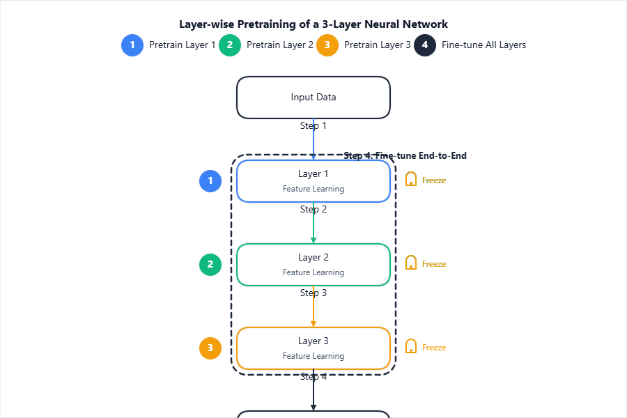
large vertical block diagram illustrating a 3-layer neural n

The diagram above shows the step-by-step process of greedy layer-wise pre-training.

[!TIP]

Draw the flowchart and label each step in your answer—easy marks!

Benefits and Limitations

Benefits	Limitations
Mitigates vanishing/exploding gradients	Adds to the overall training time
Provides better weight initialization	Unsupervised pre-training may not always help
Makes deep training more stable	Now largely replaced by better inits/functions
Less likely to get stuck in poor local minima	Needs separate unsupervised data sometimes

2. Better Activation Functions

Limitations of Traditional Activation Functions

[!IMPORTANT]

Traditional activation functions like sigmoid or tanh suffer from gradient saturation (vanishing gradient), slow convergence, and computational inefficiency.

Sigmoid: Output saturates at 0 or 1 leading to vanishing gradients.
Tanh: Same issue; although output range is $(-1, 1)$.

Modern Activation Functions

ReLU (Rectified Linear Unit)

[!IMPORTANT]

Definition: The ReLU function is defined as $f(x) = \max(0, x)$.

Easy to compute; avoids vanishing gradients for $x > 0$.
Allows faster and more effective training of deep networks.

Leaky ReLU, Parametric ReLU

[!IMPORTANT]

Leaky ReLU: $f(x) = \max(\alpha x, x)$ where $\alpha$ is a small value like 0.01 ($\alpha$ prevents neurons from "dying").

Parametric ReLU (PReLU): Like Leaky ReLU, but $\alpha$ is learned during training.

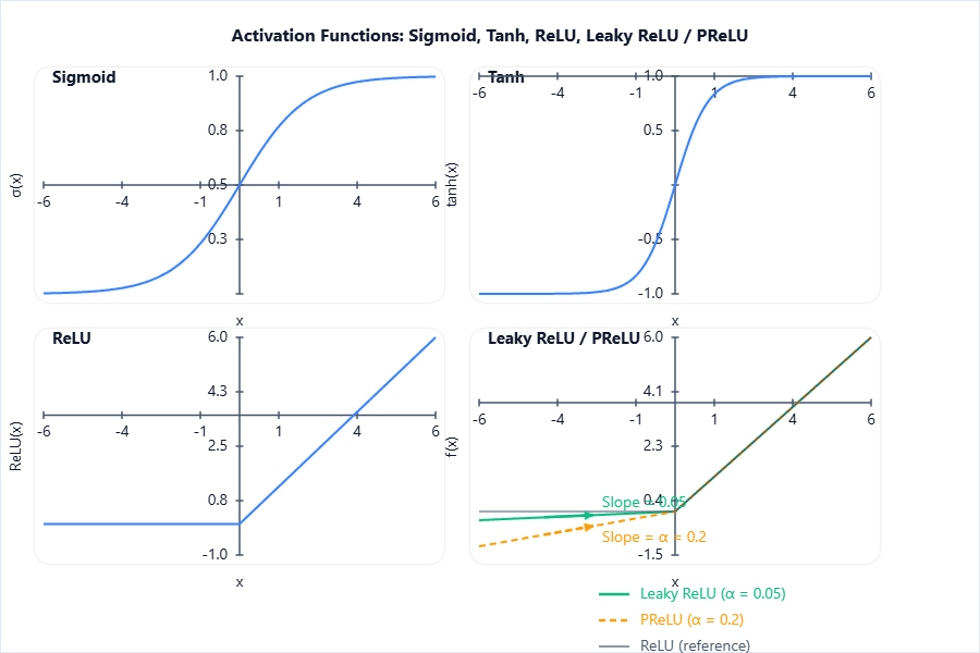
Four sub-plots showing the function curves for Sigmoid, Tanh

The above plot visually compares activations’ shapes and their treatment of negative inputs.

ELU, SELU

[!IMPORTANT]

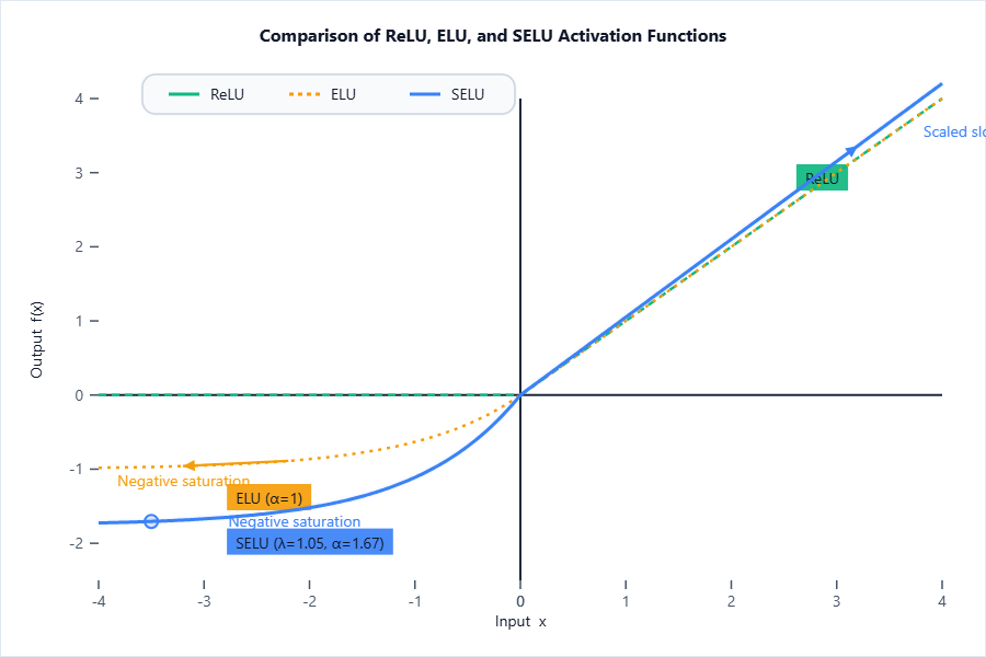
ELU: $f(x)=x$ if $x > 0$; $\alpha (e^x - 1)$ if $x \leq 0$ (smooth, nonzero mean helps learning).

SELU: Scaled ELU, with scale parameters for self-normalizing properties in deep networks.

ELU and SELU curves compared to ReLU—SELU curve shows slight

Swish, Mish

Swish: $f(x) = x \cdot \sigma(\beta x)$; smooth and non-monotonic.
Mish: $f(x) = x \cdot \tanh(\ln(1+e^x))$.

Comparison Table

Activation	Formula	Gradient Issues?	Learnable Params	Output Range
Sigmoid	$\frac{1}{1+e^{-x}}$	Yes (saturates)	No	(0, 1)
Tanh	$\tanh(x)$	Yes	No	(-1, 1)
ReLU	$\max(0, x)$	“Dead units”	No	[0, $\infty$)
Leaky ReLU	$\max(\alpha x, x)$	Less	$\alpha$ fixed	(-$\infty$, $\infty$)
PReLU	$\max(\alpha x, x)$	Less	$\alpha$ learned	(-$\infty$, $\infty$)
ELU	$x$, $\alpha(e^x-1)$	Rare	$\alpha$	(-$\infty$, $\infty$)
SELU	$\lambda$ ELU	No	$\lambda,\alpha$	(-$\infty$, $\infty$)
Swish	$x\sigma(\beta x)$	No	$\beta$	(-$\infty$, $\infty$)
Mish	$x\tanh(\ln(1+e^x))$	No	No	(-$\infty$, $\infty$)

3. Better Weight Initialization Methods

Challenges in Weight Initialization

[!IMPORTANT]

Poor weight initialization can cause vanishing/exploding gradients, slow convergence, and poor local minima, especially in deep networks.

All zeros: No symmetry breaking
All large/small random: Leads to exploding or vanishing activations

Popular Methods

Random and Zero Initialization

Random: Small values from Gaussian/uniform distributions often used.
Zero: If all weights are zero, all neurons learn the same features (bad).

Xavier/Glorot Initialization

[!IMPORTANT]

Definition: Xavier initialization chooses weights to keep the variance of activations and gradients the same across layers.

Derivation:

Let $n_{in}$ and $n_{out}$ be input and output neuron counts of a layer.

For a layer with input $x$ and weights $W$:

Want: $\mathrm{Var}[y^{(l)}] = \mathrm{Var}[y^{(l-1)}]$, where $y^{(l)} = W x$

Set

$$ W \sim \mathcal{U}\left(-\sqrt{\frac{6}{n_{in} + n_{out}}},\ \sqrt{\frac{6}{n_{in} + n_{out}}}\right) $$

or for normal distribution,

$$ W \sim \mathcal{N}\left(0,\ \frac{2}{n_{in} + n_{out}}\right) $$

$$\boxed{W \sim \mathcal{U}\left(-\sqrt{\frac{6}{n_{in} + n_{out}}},\ \sqrt{\frac{6}{n_{in} + n_{out}}}\right)}$$

He Initialization

[!IMPORTANT]

Definition: He initialization (for ReLU activations) adapts Xavier for cases where output is mostly $0$: weights are sampled as

Derivation:

$$ W \sim \mathcal{N}\left(0, \frac{2}{n_{in}}\right) $$

$$ W \sim \mathcal{U}\left(-\sqrt{\frac{6}{n_{in}}},\ \sqrt{\frac{6}{n_{in}}}\right) $$

$$\boxed{W \sim \mathcal{N}\left(0, \frac{2}{n_{in}}\right)}$$

Impact on Training Deep Networks

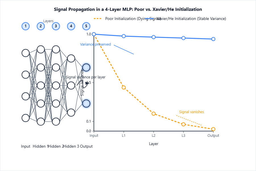
Simple 4-layer MLP, two curves: one with poorly initialized

The diagram contrasts variance propagation with poor vs. good initialization.

[!TIP]

When solving a numerical on weight initialization, always state formula, substitute $n_{in}$ and $n_{out}$, show ranges/values.

4. Learning Vectorial Representations of Words

Word Embeddings: Definition and Need

[!IMPORTANT]

Word embedding is a learned mapping of words to continuous-valued vectors that capture semantic and syntactic relationships.

Needed to convert text (categorical) to a form usable by neural networks.
Embedding vectors preserve similarity: “king” - “man” + “woman” ≈ “queen”.

Methods to Learn Word Vectors

Word2Vec

Neural model that learns vectors so that words used in similar contexts have similar vectors.

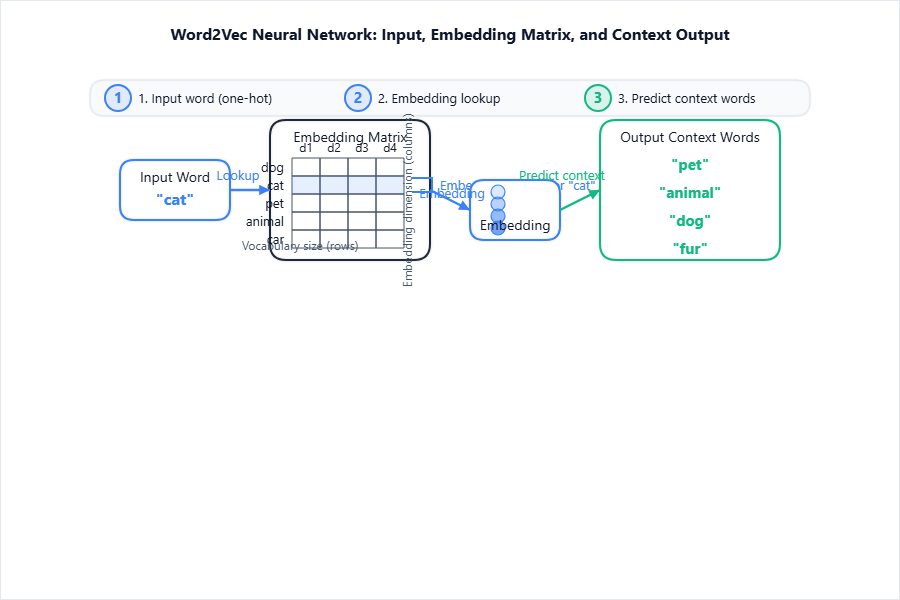
Simple neural net diagram for Word2Vec with input (“cat”), o

The diagram shows Word2Vec’s mapping: input word to 1-hot, to vector, then output probabilities.

GloVe

Counts-based: Learns embeddings so word vector dot products predict log co-occurrence counts.

CBOW and Skip-gram models

CBOW: Predicts a word from its context window.
Skip-gram: Predicts context words from a given target word.

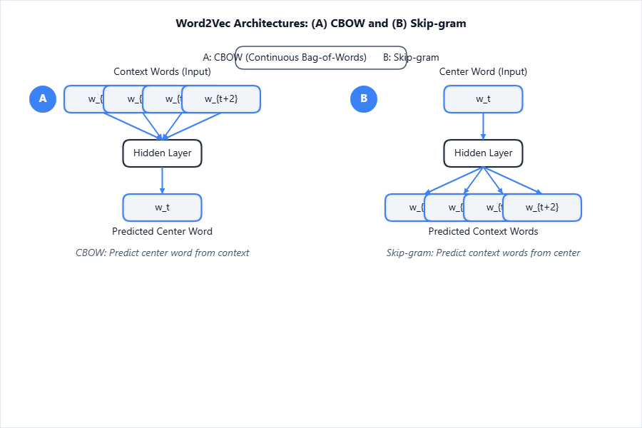
Two diagrams. (A) CBOW—context words as inputs to hidden lay

The diagrams demonstrate how CBOW and Skip-gram differ in prediction direction.

Applications of Word Vectors

Sentiment analysis, machine translation, search, chatbots, analogical reasoning.

5. Convolutional Neural Networks (CNNs)

Basic Architecture and Principles

[!IMPORTANT]

CNNs are deep networks specialized for processing data with a grid-like structure, e.g., images.

Use convolutional layers to automatically extract spatial features.
Stack convolution, pooling, and fully-connected layers.

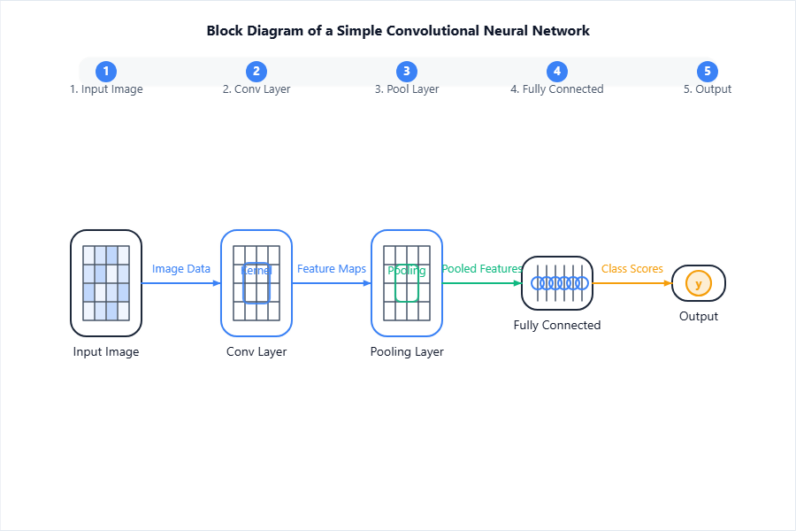
Block diagram—Input image → stacked Conv + Pool (with kernel

Shows typical CNN pipeline from image to classification.

Components of CNN

Component	Function
Convolutional Layer	Applies filters to extract local features
Pooling Layer	Downsamples feature maps, reduces spatial dimension
Fully Connected Layer	Combines high-level features for final prediction

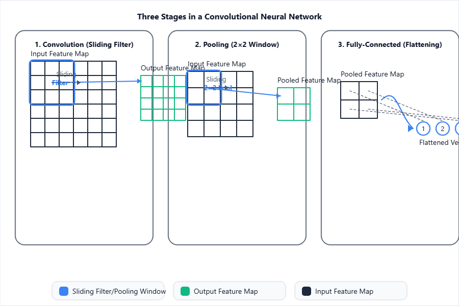
Three panel figure showing (1) Convolution (sliding filter),

Key Operations

Convolution Operation

[!IMPORTANT]

Convolution in CNNs means sliding a filter matrix $K$ over input $X$, computing

$$ > Y(i, j) = \sum_m \sum_n X(i+m, j+n) K(m, n) > $$

Numerical Example:

Given $X$ (3×3):

$\begin{bmatrix}1 & 2 & 0 \\ 4 & 2 & 1 \\ 1 & 1 & 0\end{bmatrix}$

Kernel $K$ (2×2):

$\begin{bmatrix}1 & 0 \\ 0 & -1\end{bmatrix}$

Perform convolution (no padding, stride 1):

Top-left: $1*1 + 2*0 + 4*0 + 2*(-1) = 1+0+0-2 = -1$
Top-middle: $2*1 + 0*0 + 2*0 + 1*(-1) = 2+0+0-1 = 1$
Middle-left: $4*1 + 2*0 + 1*0 + 1*(-1) = 4+0+0-1 = 3$
Middle-middle: $2*1 + 1*0 + 1*0 + 0*(-1) = 2+0+0-0 = 2$

Output feature map (2×2):

$\begin{bmatrix}-1 & 1\\ 3 & 2\end{bmatrix}$

Pooling Operation

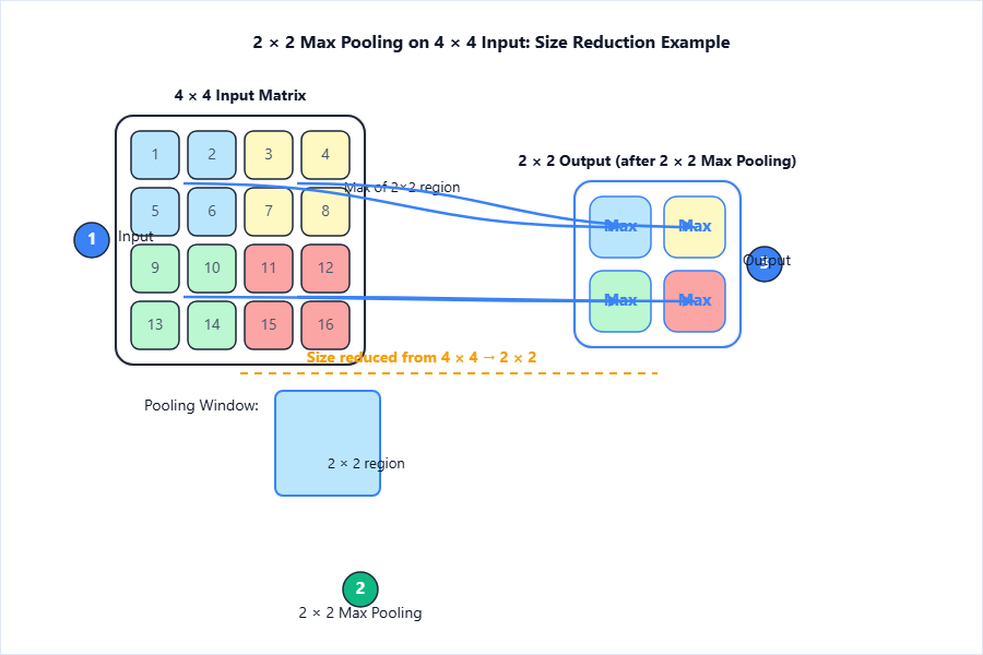
Max or Average Pooling: Replaces a patch with its max/avg, reduces computations.

4 × 4 input undergoing 2 × 2 max pooling, outputting 2 × 2 m

6. LeNet

Architecture Overview

Consists of input image, two convolutional + pooling layers, followed by two fully-connected layers and an output.

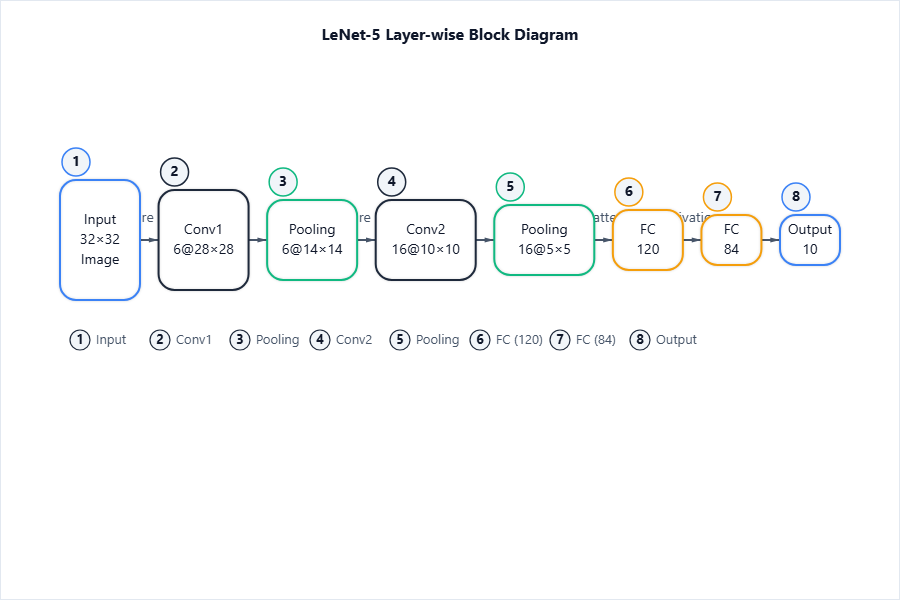
Layer-wise blocks for LeNet-5: Input (32×32 image) → Conv1 (

Classic LeNet-5 schematic, showing all dimensions and flows.

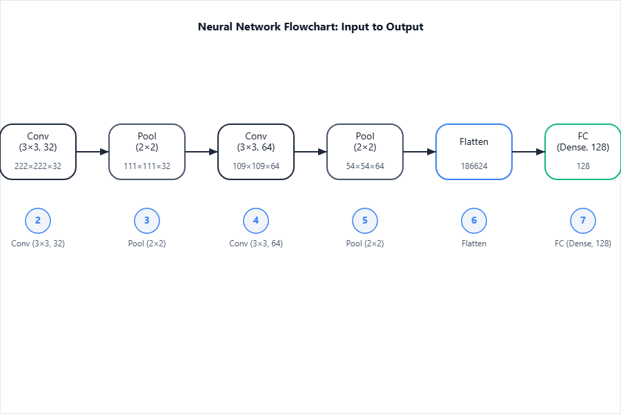
Layer-wise Structure and Data Flow

Flowchart showing sequence: Input → Conv → Pool → Conv → Poo

Applications and Significance

Pioneered deep learning for document/image recognition (e.g., digit recognition).
Underpins modern CNN architectures.

7. AlexNet

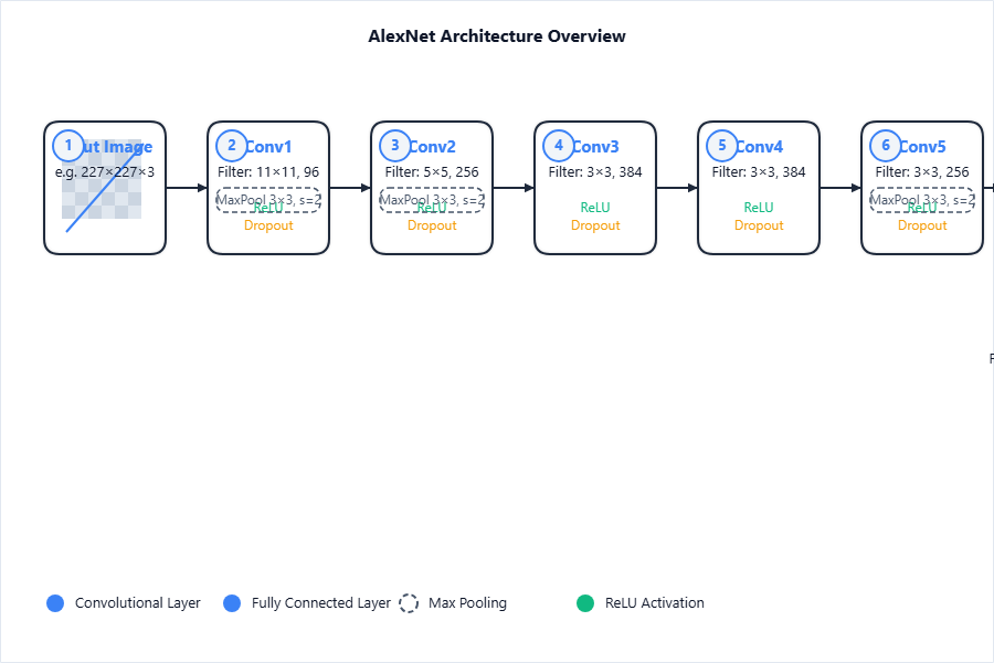
Architecture and Key Innovations

Detailed AlexNet diagram: Input image → five convolutional l

Used ReLU, Dropout, Local Response Normalization.
First large deep net for high-performance on ImageNet (~60 Million params).

Comparison to LeNet

Feature	LeNet	AlexNet
Year	1998	2012
Layers	7 (2 conv)	8 (5 conv)
Input size	32×32	224×224
Activation	Sigmoid/tanh	ReLU
Pooling	Average	Max
Regularization	N/A	Dropout
Dataset	MNIST	ImageNet
Impact	Proof-of-concept	Sparked deep learning boom

Role in ImageNet Challenge

Reduced top-5 error rate from 26% to 15%.
Demonstrated the power of deep learning at scale.

8. ZF-Net

Motivation and Improvements over AlexNet

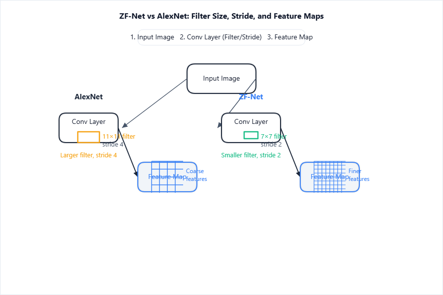
ZF-Net (Zeiler & Fergus) refined AlexNet by visualizing feature maps, adjusting filter sizes and stride for better accuracy.

ZF-Net vs AlexNet—showing 7×7 filter (not 11×11), stride cha

Architecture Highlights

Five convolutional layers (like AlexNet), but with smaller first layer filters.
Visualizes and tunes features at each layer.

9. VGGNet

Architectural Innovations

Used only 3×3 convolutional filters, increasing depth (up to 19 layers).
Stacked more layers for greater abstraction.

Block diagram: Input → [Conv 3×3] ×2 → Pool → [Conv 3×3] ×2

Depth and Use of Small Filters

Many layers with identical small filters dramatically improved accuracy with fewer parameters per layer.

10. GoogLeNet

Inception Module Explanation

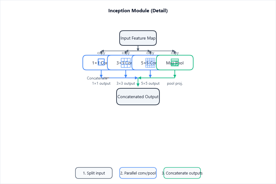
Inception module detail—input flows in parallel into 1×1, 3×

Each module computes multiple scaled convolutions/pooling in parallel.

Network Architecture

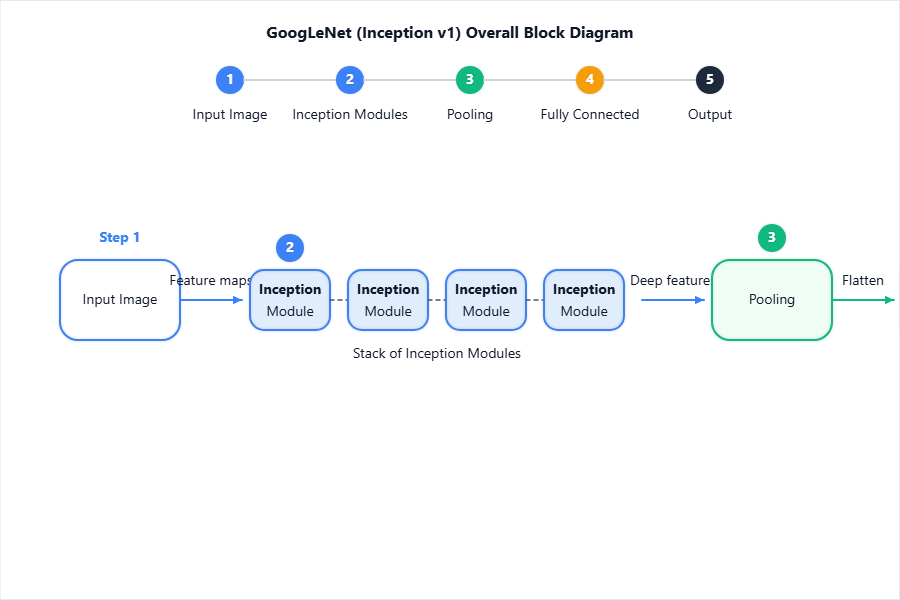
Overall GoogLeNet block diagram: Input → stack of Inception

22 layers, ~5M parameters, won ILSVRC 2014.

11. ResNet

Skip Connections/Residual Blocks

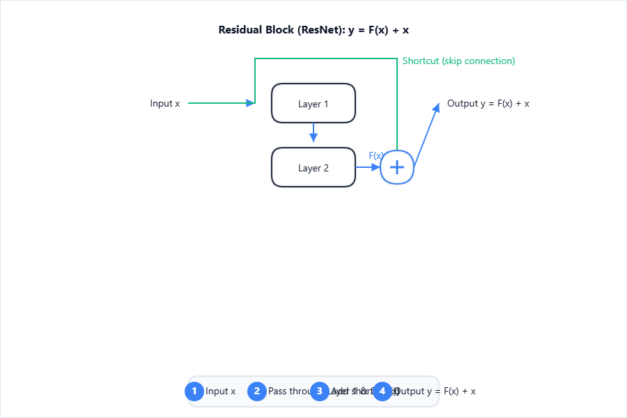
Residual (ResNet) block: input x, passes through two stacked

Skip connections add input directly to layer output: $y = F(x) + x$.

ResNet Architecture Overview

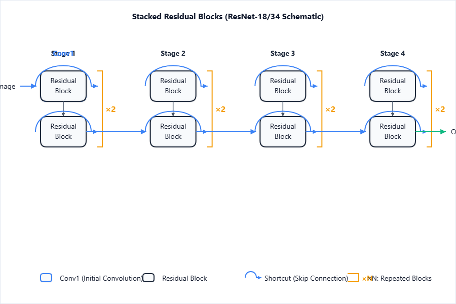
Stacked residual blocks with shortcut arrows, e.g., ResNet-1

Enables training of extremely deep networks, e.g., 50/101/152 layers.

Impact on Training Deeper Networks

Solved vanishing gradient problem; deeper networks became feasible and performed better.

12. Visualizing Convolutional Neural Networks

Techniques for Visualizing Learned Features

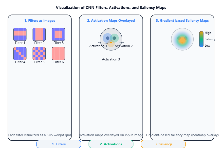
Three panels: (1) Filters visualized as images, (2) Activati

Feature maps, filter visualization, saliency maps, deconvolution, Guided Backprop.

Importance of Visualization

Helps interpret model’s focus and decisions, identifies what is being learned.

13. Guided Back Propagation

Principle and Steps

[!IMPORTANT]

Guided backpropagation visualizes which pixels most influence a network’s output by modifying backward ReLU to only propagate positive gradients.

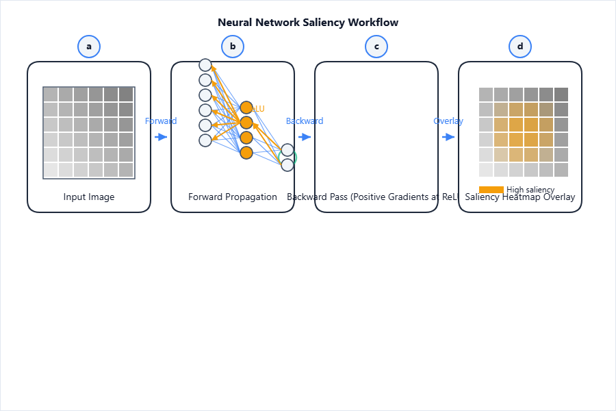
Workflow showing (a) input, (b) forward propagate, (c) backw

Principle: Only positive activations and gradients propagate, highlighting parts of the input that drive the classification.

Application to Interpretability

Used for debugging, understanding CNN behavior, and feature localization.

14. Deep Dream

Purpose and Method

[!IMPORTANT]

Deep Dream is an algorithm that modifies an image to maximally activate certain network features, creating dream-like outputs.

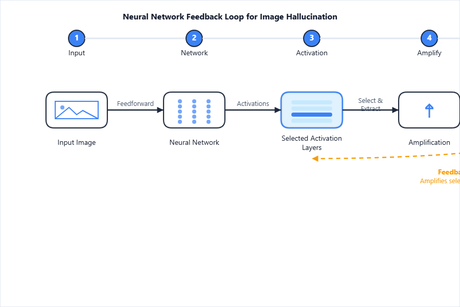
Input image, feedback loop amplifies selected activation lay

“Dreams” are produced by iteratively adjusting input to amplify higher-level features visualized in the image.

Example Outputs (Brief)

Images with over-interpreted textures and repeated motifs (e.g., dogs, buildings).

15. Deep Art

Concept and Algorithm

[!IMPORTANT]

Deep Art (neural style transfer) blends content of one image with the style of another using optimization of network activations.

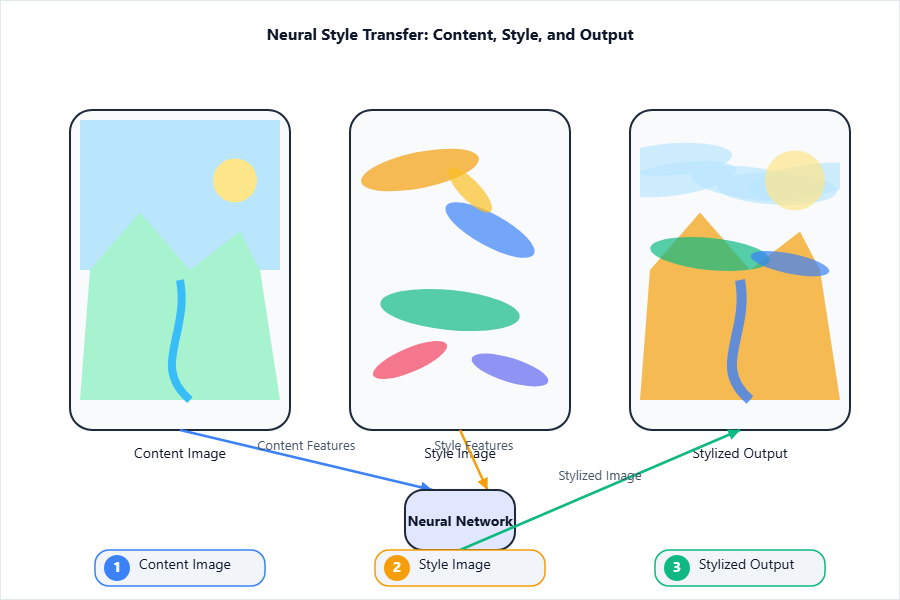
Content image, style image, and neural net output that mimic

Algorithm: Optimize an image to have low loss for both content features (from one image) and style features (from another).

Artistic Applications

Produces stylized paintings, video, animations; used in design, film, and apps.

16. Recent Trends in Deep Learning Architectures

Hybrid Models

Networks combine CNNs (vision) and RNNs (sequences), or use attention (for relations/context).
E.g., image captioning: CNN encodes image, RNN generates caption.

Advancements: EfficientNets, Transformers, Self-Attention

EfficientNets: Use compound scaling to balance depth, width, and resolution.
Transformers: Attention mechanisms without recurrence/convolution; foundational for language models.
Self-Attention: Each input attends to all others, powerful for sequence modeling.

Overview of AutoML, NAS

AutoML: Automated design and tuning of neural networks.
NAS (Neural Architecture Search): Algorithms design optimal network topologies, outperforming manual architecture design.

[!TIP]

Answer subtopics with diagrams and formulae for full marks. Tabulate whenever comparisons are possible. Always include visual/algorithmic descriptions for model architecture topics.